library(ggplot2)
library(dplyr)
library(lterdatasampler)
library(knitr)Full Workflow
Start by loading packages.
Then load in the data.
data(pie_crab)Create a table of summary statistics.
# create summary table
summ_tble <- pie_crab %>%
  select(site, size, latitude) %>%
  group_by(site) %>%
  summarise(mean_size = mean(size),
            latitude = unique(latitude),
            sd_size = sd(size))

# make the table print with a caption
summ_tble %>%
kable()| site | mean_size | latitude | sd_size |
|---|---|---|---|
| BC | 16.197297 | 42.2 | 4.814463 |
| CC | 16.815185 | 41.9 | 2.054689 |
| CT | 14.691515 | 41.3 | 2.357521 |
| DB | 15.604000 | 39.1 | 2.119959 |
| GTM | 12.403214 | 30.0 | 1.804449 |
| JC | 15.274667 | 39.6 | 2.722022 |
| NB | 17.140345 | 41.6 | 2.288182 |
| NIB | 13.292000 | 33.3 | 2.419173 |
| PIE | 18.503929 | 42.7 | 2.296058 |
| RC | 12.491600 | 34.7 | 2.344991 |
| SI | 9.854333 | 31.4 | 1.790097 |
| VCR | 16.335667 | 37.2 | 2.938512 |
| ZI | 12.063714 | 34.0 | 2.009251 |
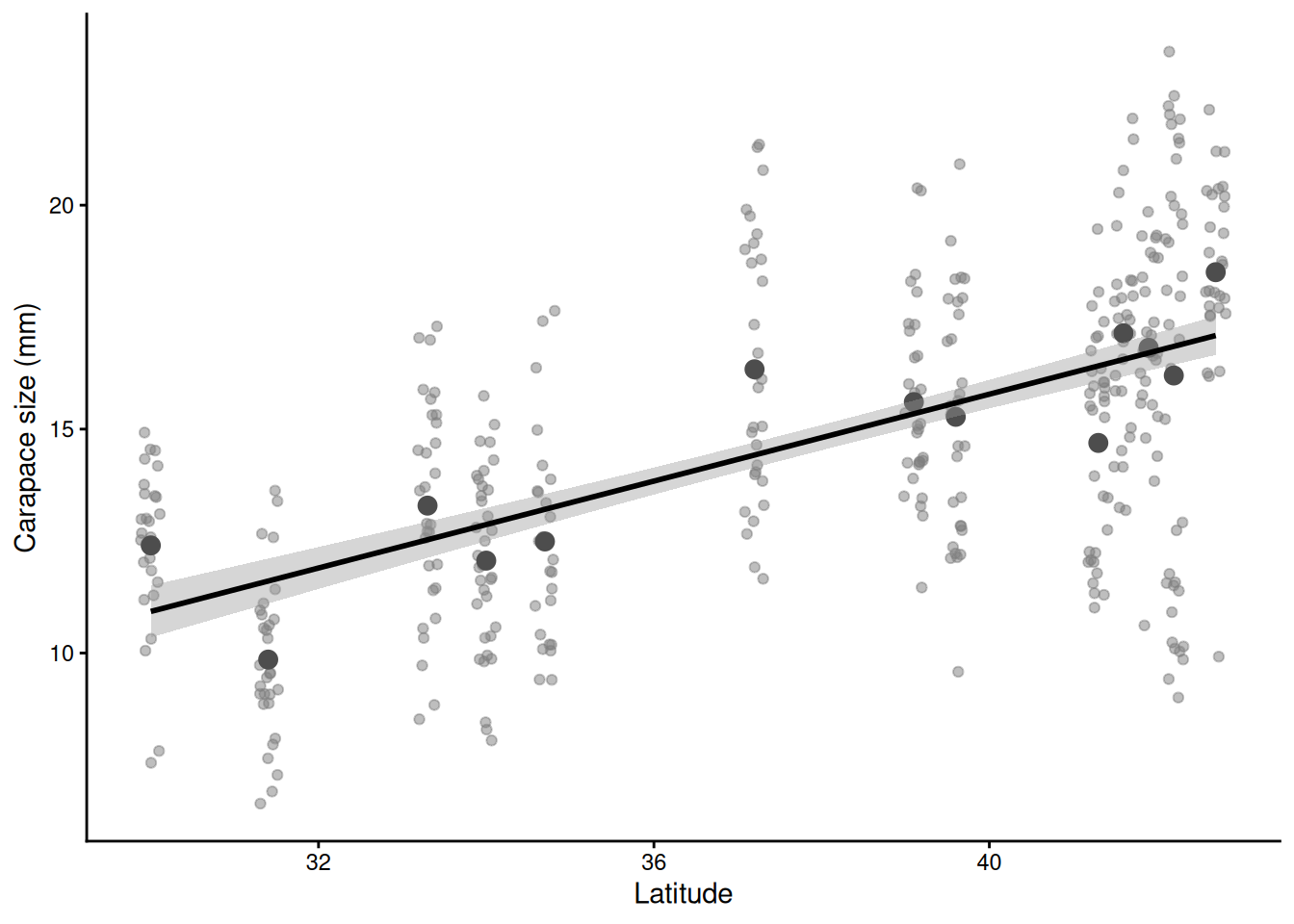
Then plot it.
ggplot(data = pie_crab,
       aes(x = latitude, y = size)) +
  geom_jitter(color = "grey50", alpha = 0.5) +
  geom_point(data = summ_tble,
             aes(x = latitude, y = mean_size),
             color = "grey30", size = 3) +
  geom_smooth(formula = y~x, method = "lm",
              color = "black") +
  labs(x = "Latitude", y = "Carapace size (mm)") +
  theme_classic()